Custom models: your own precision matrix
Source:vignettes/articles/custom-models.Rmd
custom-models.RmdIf a model is not built in, you can supply the dependency matrix
and the constant vector
yourself with ngvb_custom(). The engine then forms
,
owns its normalizing constant, and ng.check() and
ngvb() work exactly as before.
For areal data the natural custom model is the simultaneous
autoregression (SAR), which uses
with
a row-standardised adjacency. This is worth stressing: among areal
models, the SAR is the one you build through ngvb_custom().
A proper CAR, or the intrinsic besag/ICAR family, cannot be written as a
custom
of this kind, because their precisions are specified conditionally or
intrinsically rather than through a whitening operator with a fixed
sparsity pattern. The intrinsic besag model is instead available by
auto-detection, as in Areal data, and there is
no way to hand it to ngvb_custom() as a bespoke operator.
So for a custom areal model, think SAR.
Unlike the intrinsic besag effect, the SAR mixing variables live on the counties themselves, so we can map them directly.
We reuse the Columbus burglary data from Areal data:
library(sf); library(spdep)
map  <- st_read(system.file("shapes/columbus.gpkg", package = "spData"), quiet = TRUE)
d    <- st_drop_geometry(map[, c("CRIME", "HOVAL", "INC")])
d$s  <- seq_len(nrow(d))
nb   <- poly2nb(map)
Wadj <- Matrix::sparseMatrix(i = rep(seq_along(nb), lengths(nb)), j = unlist(nb), x = 1)
Here is the full definition, and each argument is explained just below it.
W      <- Matrix::Diagonal(x = 1 / rowSums(Wadj)) %*% Wadj    # row-standardise
N      <- nrow(W)
eigenv <- Re(eigen(as.matrix(W), only.values = TRUE)$values)

op_sar <- ngvb_custom(
  D = function(theta) {
    rho <- exp(theta[2]) / (1 + exp(theta[2]))
    sqrt(exp(theta[1])) * (Matrix::Diagonal(N) - rho * W)
  },
  h        = rep(1, N),
  ntheta   = 2,
  logprior = function(theta) {
    rho <- exp(theta[2]) / (1 + exp(theta[2]))
    stats::dnorm(theta[1], 0, 3, log = TRUE) + log(rho) + log(1 - rho)
  },
  lognc = function(theta, Vinv) {
    rho <- exp(theta[2]) / (1 + exp(theta[2]))
    0.5 * N * theta[1] + sum(log(1 - rho * eigenv)) +
      0.5 * sum(log(Vinv)) - 0.5 * N * log(2 * pi)
  })
The arguments are:
-
D = function(theta)builds the dependency matrix as a sparseMatrix. Its rows are the driving-noise terms and its columns are the latent nodes. Heretheta[1]is the log precision andtheta[2]is the internal (unconstrained) version of , mapped into by the logistic function. INLA works on this internal scale, which is why the transform appears insideD. -
his the constant vector with , and recovers the Gaussian model. For a discrete areal model there is one innovation per node, sohis a vector of ones. -
nthetais the number of hyperparameters that INLA estimates, here two. -
logprior = function(theta)is the log prior density of the hyperparameters, written on the internal scale and including any change-of-variables Jacobian. This is the piece INLA adds to the log-posterior for . In this example there is a prior on the log precision, and a uniform prior on ; after the logistic transform the uniform density contributes the Jacobian term . If you omitlogprior, an independent on each internal hyperparameter is used. -
lognc = function(theta, Vinv)is optional but recommended when can get close to singular, as it does here when approaches one. It returns the log normalizing constant of the conditional Gaussian density, , and it receivesVinvso that the -dependent part of the determinant is included. For the SAR the log-determinant has the closed form , using the eigenvalues of , which is both fast and stable near the boundary. Whenlogncis omitted, the engine computes the determinant generically, which is fine for well-conditioned operators.
A couple of practical notes. D, logprior,
and lognc are evaluated in a separate R process where only
the base packages are attached, so any non-base function must be
namespace-qualified, which is why the code writes
Matrix::Diagonal and stats::dnorm, and uses
exp(t)/(1+exp(t)) rather than plogis. The data
those functions reference, such as W and
eigenv, is captured automatically.
With the operator defined, fit the Gaussian SAR through the same engine and then extend it:
LGM  <- inla(CRIME ~ 1 + HOVAL + INC + f(s, model = ngvb_rgeneric(op_sar)),
             data = d, control.compute = list(config = TRUE))
LnGM <- ngvb(LGM, components = list(s = op_sar), verbose = FALSE)
plot(LnGM)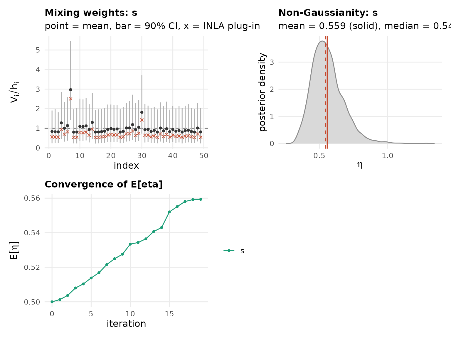
Because the SAR weights live on the counties, we can put them straight back on the map. Low values are yellow and high values are red, so the reddest counties are where the model added the most flexibility, meaning the largest local departures from the smooth spatial field:
areal.plot(map, LnGM$V$s, title = "V")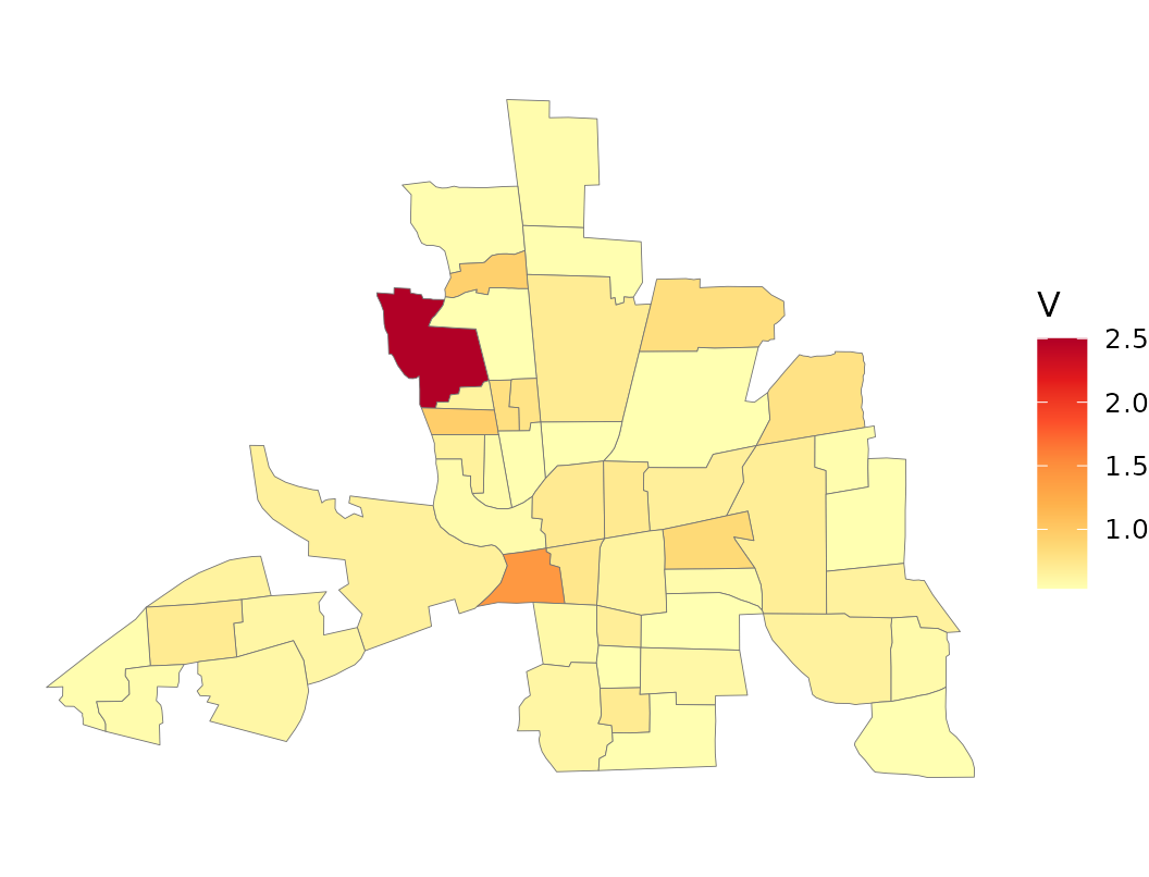
bayes.factor(LnGM, n.samples = 30, seed = 1)
#> Bayes factor (non-Gaussian vs Gaussian): 8.53
#>   log10 BF = 0.93  (substantial)
#>   weight ESS = 24.8 of 30 draws
That is the whole custom interface. Give ngvb_custom() a
function D(theta) and a vector h, optionally a
prior and a normalizing constant, and any Gaussian model whose precision
factors as
becomes a latent non-Gaussian one.
Using operators from the ngme2 package
The ngme2 package is a good source of ready-made dependency matrices for models beyond ngvb’s own registry (general AR(p), tensor-product and bivariate operators among them). Its operator objects expose , the dependency matrix D you need, as a function of a hyperparameter, and . For an AR(1) field, for example:
ngme_ar1 <- ngme2::ar1(1:100)

op_ar1_ngme2 <- ngvb_custom(
  D = function(theta) sqrt(exp(theta[1])) * ngme_ar1$update_K(theta[2]),
  h        = ngme_ar1$h,
  ntheta   = 2,
  logprior = function(theta) {
    stats::dnorm(theta[1], 0, 3, log = TRUE) +   # precision: your choice
    stats::dnorm(theta[2], 0, 1, log = TRUE)     # matches ngme2's own prior_normal(0, 1) on theta_K
  })
theta[1] is your own added precision hyperparameter;
theta[2] is passed straight through to ngme2’s
update_K, which applies its own internal transform to
it.