library(ngvb)
library(ggplot2)
library(INLA)     # ngvb uses INLA as a backend; attach it to call inla() directly
Overview
A latent Gaussian model (LGM), the workhorse of R-INLA, places a Gaussian prior on a latent field: a random walk, an autoregression, a spatial effect, or a set of random effects. That prior is convenient but rigid, because it assumes Gaussianity everywhere. Real data often break this assumption in just a few places, such as a sudden jump in a time series, one outlying subject, a sharp boundary between regions, or a local hotspot in space. A Gaussian model then has to compromise. It either over-smooths the interesting feature or inflates the variance everywhere to accommodate it.
ngvb relaxes that single assumption. It keeps everything
you already have, the same INLA model and the same code, and replaces
the Gaussian driving noise with a heavier-tailed one. The result adds
flexibility only where the data ask for it and falls back to the
Gaussian model everywhere else. Two functions do the work, and both take
an ordinary inla fit that was run with
control.compute = list(config = TRUE):
-
ng.check(fit)asks whether you should relax the Gaussian assumption, and where. -
ngvb(fit)fits the non-Gaussian extension.
The model in one paragraph
Every LGM writes its latent field
through a model-specific dependency matrix
that turns
into independent Gaussian increments,
For a
random walk
,
for an autoregression
,
and so on. Equivalently, the Gaussian field has precision
. The
non-Gaussian model keeps the same
but lets each increment have its own variance
,
The mixing variables
carry the local flexibility. Where
the model is Gaussian, and where
is inflated the increment is allowed to be unusually large. A single
non-Gaussianity parameter
controls how far
may stray from
,
and
is exactly the Gaussian model. Conditional on
the field is still Gaussian, with precision
ngvb fits the model with a short variational-Bayes loop
that repeatedly calls INLA with
fixed and then updates
and
.
The prior on
is an exponential (a penalised-complexity prior with rate
alpha.eta, default
)
that shrinks toward the Gaussian model, so non-Gaussianity has to earn
its place. Increase alpha.eta for stronger shrinkage.
Two variational algorithms are available. The default,
method = "SVI", is a structured mean-field scheme that
updates
and
in turn, and it is the more reliable choice. The alternative,
method = "SCVI", integrates
out of the
update analytically and so converges in fewer iterations, but its
collapsed marginal can over-shrink a weak yet genuine effect all the way
to the Gaussian model.
Which models and likelihoods are supported
The non-Gaussianity in ngvb lives entirely in the latent
field, on its driving noise, and never touches the observation model. So
every INLA likelihood is available: Gaussian, Poisson,
binomial, negative binomial, survival families, and the rest all work
unchanged. You just fit your LGM as usual and hand it to
ng.check() or ngvb().
The latent components split into three groups.
Detected automatically. If your fit uses one of
these, ngvb() and ng.check() find it with no
extra arguments: iid, rw1, rw2,
ar1, besag (the intrinsic CAR),
spde / spde2 (Matern fields), and
seasonal. Each of these is a single operator applied to
independent noise, so it has the dependency matrix
the method needs.
Added by hand. Some models are not auto-detected but
are still described by
,
so you can build them with ngvb_operator() which expects
the matrix
,
the vector
.
This covers the simultaneous autoregression (sar) or the
Ornstein-Uhlenbeck process (ou). It is also possible to use
the matrices and operators of the ngme2 package to define
the LnGM; both are covered in Custom
models.
Not compatible. Some components are not a single
operator applied to one field, and the method does not apply to them.
The main cases are the additive spatial models bym,
bym2, besag2 (a latent field that is a sum of
parts), the conditionally specified besagproper, the copy
and mixture constructions generic1, generic2,
generic3, copy, scopy,
z, the measurement-error models mec,
meb, and the nonlinear-covariate effects sigm,
revsigm, log1exp, logdist. For an
additive model such as bym, the practical fix is to split
it into its besag and iid parts as two
separate f() terms, which ngvb() then extends
jointly.
Priors carry over the same way: pc.prec,
loggamma, and normal precision priors on the
original f() term are read from the fit and reused
automatically; anything else falls back to a default prior with a
warning.
A time series with jumps
jumpts is a series that is smooth apart from two abrupt
jumps.
ggplot(jumpts, aes(x, y)) +
  geom_line(colour = "grey70") +
  geom_point(colour = "grey30", size = 1.3) +
  labs(title = "jumpts", x = "time", y = "y") +
  theme_minimal(base_size = 12)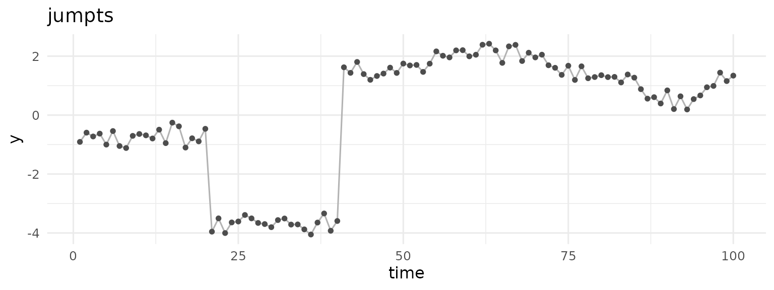
A first-order random walk models the series through its increments, which is the operator with the first-difference matrix. A Gaussian RW1 forces every increment to share the same variance, so it cannot tell a jump from ordinary noise. Fit it with INLA:
Now check whether the latent Gaussian assumption holds:
check <- ng.check(LGM, compute.fixed = FALSE)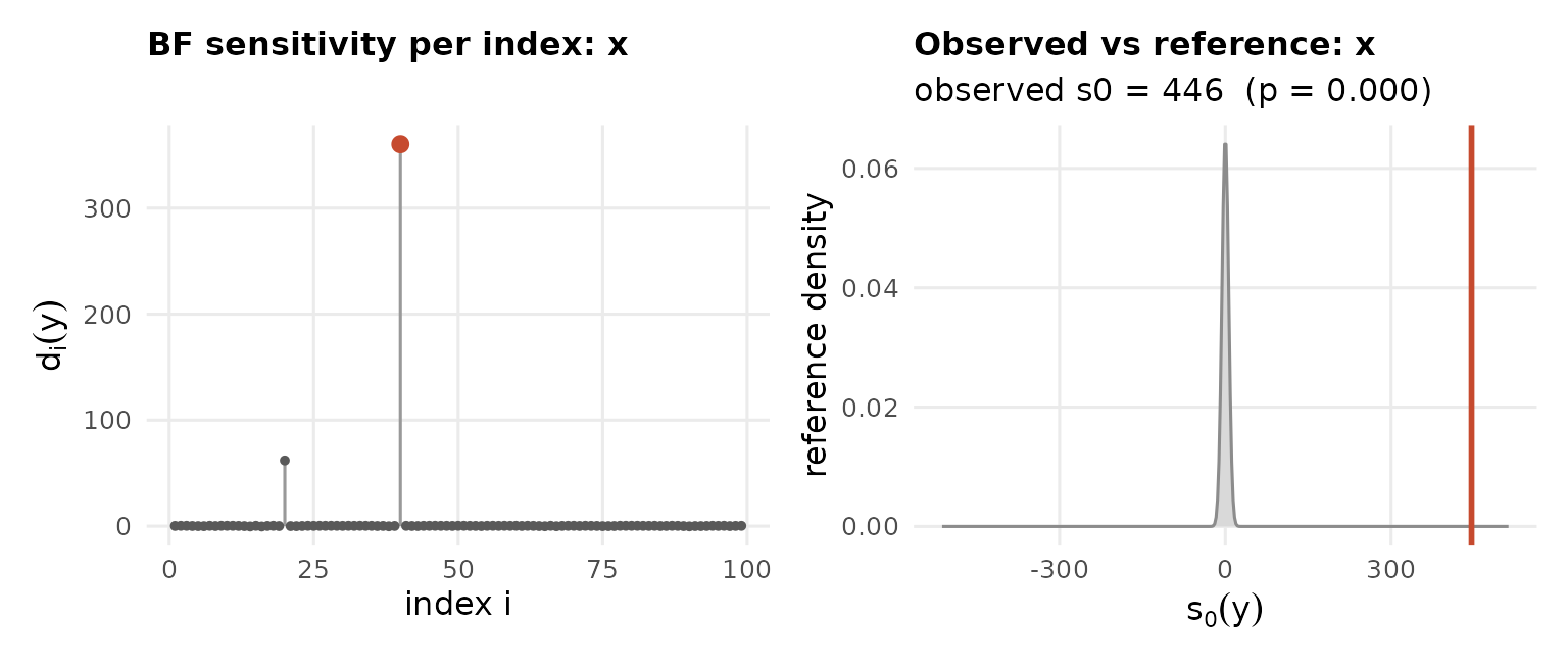
The left panel is the per-index sensitivity , which measures how much the evidence would improve if increment were allowed to be non-Gaussian. It spikes at the two jumps. The right panel compares the observed overall sensitivity (the vertical line) against the distribution it would have under a truly Gaussian field (the grey curve). The observed value sits far out in the tail, with , so the Gaussian RW1 is inadequate and we know exactly where.
Now we extend it to non-Gaussianity. The model is auto-detected, so this is a single call:
LnGM <- ngvb(LGM)
#> Components: x [rw1]
#> ngvb: converged after 24 iteration(s);  E[eta] = 3.742
plot(LnGM)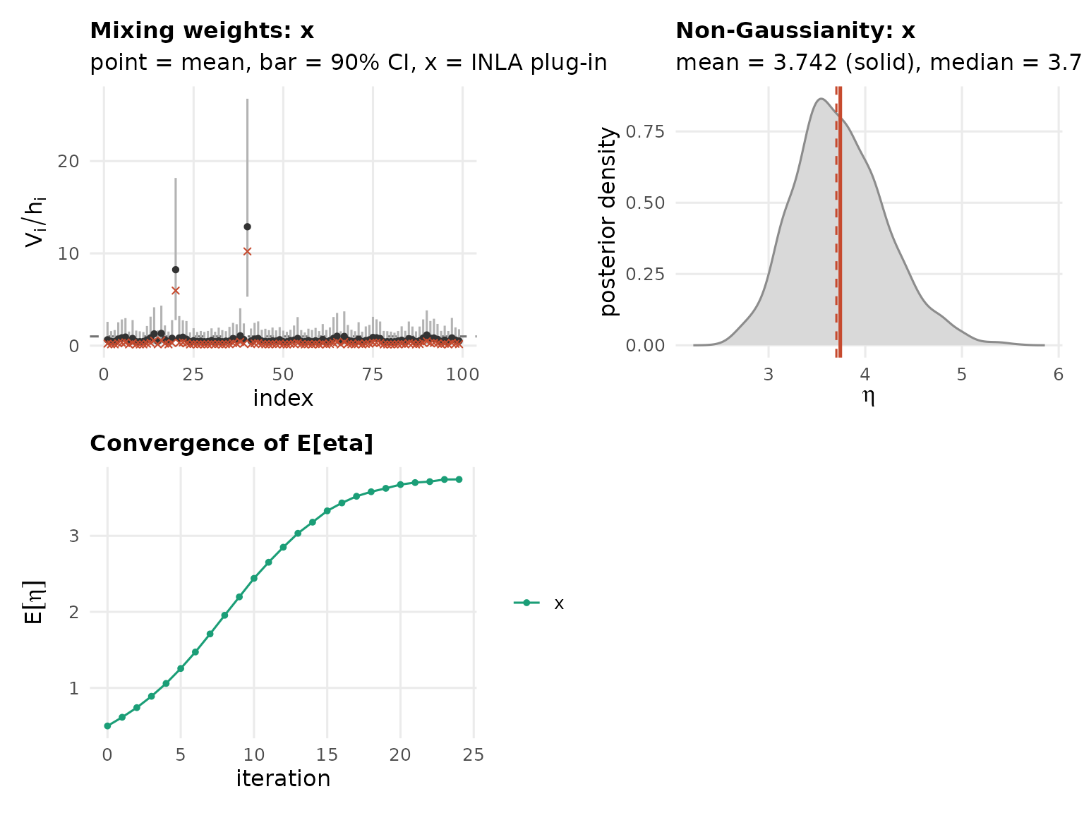
For each component the plot shows the mixing weights (the posterior mean with a 90 percent credible interval, and a cross at the plug-in value that INLA is actually refit with, which sits a little below the mean because is right-skewed). The final panel tracks across the iterations. The mixing variables are inflated precisely at the two jumps and sit near one elsewhere, so the model bought local flexibility exactly where it was needed and stayed Gaussian in between. The non-Gaussianity parameter is clearly positive.
Beyond the point estimate, you can integrate the mixing variables V out entirely by sampling from their variational posterior and refitting the LGM at each draw. This gives the Bayes factor against the Gaussian model, and, pooled with importance weights, posterior summaries of anything the underlying inla() fit reports:
samples <- ngvb_sample(LnGM, n.samples = 30)
bayes.factor(samples)               # LnGM vs. LGM marginal-likelihood ratio
#> Bayes factor (non-Gaussian vs Gaussian): 9.96e+23
#>   log10 BF = 24.00  (decisive)
#>   weight ESS = 2.2 of 30 draws
summary(samples)                    # importance-weighted summaries, V integrated out
#> Latent non-Gaussian model, V integrated out over 30 draws
#> Bayes factor vs Gaussian model: 9.96e+23 (log10 = 24.00), weight ESS 2.2
#>
#> Fixed effects:
#>   (none)
#>
#> Hyperparameters:
#>                                              mean         sd
#> Precision for the Gaussian observations 3588.3315 13688.8103
#> Theta1 for x                               2.1162     0.4493
#>
#> Random effects:
#>   $x (100 nodes)
#>   ID    mean     sd
#> 1  1 -0.8755 0.1419
#> 2  2 -0.6634 0.1094
#> 3  3 -0.7070 0.0956
#> 4  4 -0.6998 0.0999
#> 5  5 -0.8781 0.1213
#> 6  6 -0.7240 0.1306
#>   ... 94 more row(s); use what = "random" to print in full
On the usual scale a
Bayes factor above
,
,
or
is substantial, strong, or decisive evidence for the non-Gaussian model.
Here it is far into the decisive range. The ess field is
the effective number of draws behind the estimate; if it is small, raise
n.samples.
Where to next
The same two calls carry over to every other kind of data:
-
Geostatistical data fits a Matern
(SPDE) field to pressure readings and maps, before
ngvb()is ever run, where the spatial predictions will move. -
Areal data applies the intrinsic CAR
(
besag) model to burglary rates across Columbus, Ohio. - Random intercepts and slopes treats subject-level random effects in a longitudinal growth study.
-
Custom models builds a simultaneous
autoregression by hand with
ngvb_custom(), and borrows ready-made operators from thengme2package.